3.13 Visualising Raw Data

A useful tool for investigating areas of high errors or other problems in the scan data is to visualise the raw spectral data. To inspect or read individual spectra, you can plot them from the object returned from itrax_restspectra().

itrax_spectra(filename = unz(description = "CD166_19_S1/CD166_19_S1/XRF data.zip",
                             filename = "XRF data/L000642.spe"),
              parameters = "CD166_19_S1/CD166_19_S1/Results_ settings.dfl") %>% 
  invisible()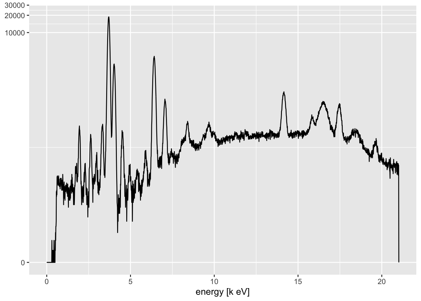

This rarely offers much insight, because we are interested in comparing multiple spectra. The itrax_restspectra() function takes its name from a similar function in the Q-Spec software from Cox Analytical Systems, Sweden. This shows a heat map of the spectra, and can be used to identify areas where particular spectral lines appear and disappear along the core. At its simplest, it can be used to produce a plot of a single scan section.

itrax_restspectra(foldername = "CD166_19_S1/CD166_19_S1/XRF data.zip",
                  parameters = "CD166_19_S1/CD166_19_S1/Results_ settings.dfl"
                  ) %>% 
  invisible()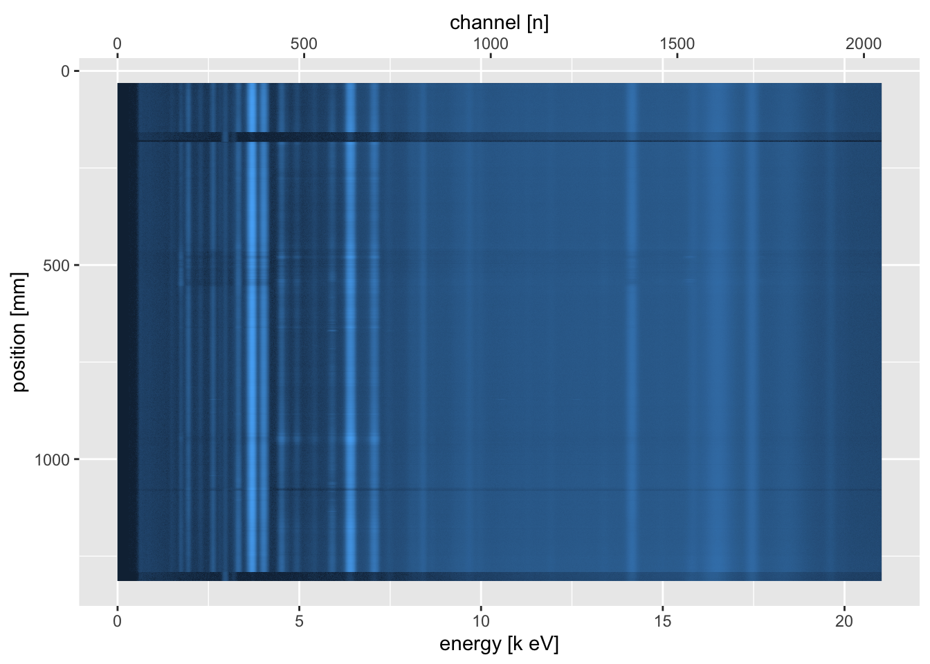

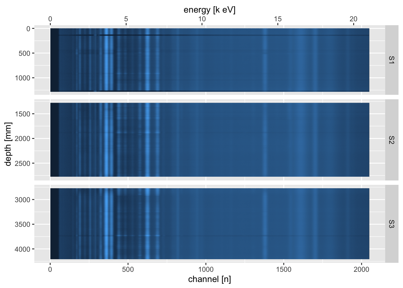
By combining all of the sections, and joining the raw spectral data with the processed data from the Results.txt (Q-Spec) output file, it can be used as a powerful diagnostic tool.

read_spectra <- function(foldername, labeltext){itrax_restspectra(foldername = foldername,
                                                                  plot = FALSE) %>%
    mutate(label = labeltext) %>%
    select(label, everything()) %>%
    mutate(filename = str_split(filename, pattern = "/") %>% sapply(., `[`, 2))}

# import the channel energy information
settings <- itrax_qspecsettings("CD166_19_S1/CD166_19_S1/Results_ settings.dfl")

# import and join them
left_join(CD166_19_xrf %>%
            select(depth, validity, filename, label) %>%
            mutate(filename = filename %>%
                     str_split(pattern = "\\\\") %>%
                     sapply(., `[`, 7)), 
          bind_rows(read_spectra(foldername = "CD166_19_S1/CD166_19_S1/XRF data.zip", labeltext = "S1"), 
                    read_spectra(foldername = "CD166_19_S2/CD166_19_S2/XRF data.zip", labeltext = "S2"),
                    read_spectra(foldername = "CD166_19_S3/CD166_19_S3/XRF data.zip", labeltext = "S3")) %>%
            mutate(label = as.factor(label)), 
          by = c("filename", "label")) %>%
  
  pivot_longer(cols = -c(depth, validity, filename, label, position),
               names_to = "channel",
               values_to = "counts") %>%
  mutate(channel = as.numeric(channel)) %>%
  select(-c("filename", "validity", "position")) %>%
  
  ggplot(aes(x = channel, y = depth, fill = counts)) +
  geom_tile() +
  scale_fill_gradient(name = "value",
                      trans = "pseudo_log",
                      low = "#132B43",
                      high = "#56B1F7",
                      labels = round) +
  scale_y_reverse(breaks = seq(from = 0, to = max(CD166_19_xrf$depth), by = 500),
                  name = "depth [mm]") +
  scale_x_continuous(name = "channel [n]",
                     sec.axis = sec_axis(trans = ~ ((. * as.numeric(settings[1,2])) + as.numeric(settings[2,2])),
                                         name = "energy [k eV]")) +
  guides(fill = "none") +
  facet_grid(rows = vars(label),
             scales = "free_y",
             space = "free_y")

rm(settings, read_spectra)