3.10 Uncertainties

The best way to quantify the uncertainties in the XRF data is in repeat measurements. The example dataset contains short sections of repeat measurements. An example might begin by reading in the repeat scan data, as below for CD166_19_S1.

CD166_19_S1_REP1 <- itrax_import("CD166_19_S1/CD166_19_S1_REP1/Results.txt") %>%
  select(any_of(c(elementsList, "position", "Mo inc", "Mo coh"))) %>%
  mutate(scan = "scan1")
CD166_19_S1_REP2 <- itrax_import("CD166_19_S1/CD166_19_S1_REP2/Results.txt") %>%
  select(any_of(c(elementsList, "position", "Mo inc", "Mo coh"))) %>%
  mutate(scan = "scan2")
CD166_19_S1_REP3 <- CD166_19_S1$xrf %>%
  filter(position >= min(c(CD166_19_S1_REP1$position, CD166_19_S1_REP2$position)) & 
           position <= max(c(CD166_19_S1_REP1$position, CD166_19_S1_REP2$position))) %>%
  select(any_of(c(elementsList, "position", "Mo inc", "Mo coh"))) %>%
  mutate(scan = "scan3")

It should then be combined into a single dataset, and finally, a function to calculate the uncertainties is called (here we use sd()). The errors package is used to create an output that can combine both the value and the associated uncertainty. It is a really neat way of working with quantities and ensures the uncertainties are correctly propagated throughout the work.

S1_reps <- list(CD166_19_S1_REP1, CD166_19_S1_REP2, CD166_19_S1_REP3) %>%
  reduce(full_join) %>%
  select(scan, position, everything()) %>%
  group_by(position) %>%
  summarise(across(any_of(c(elementsList, "Mo inc", "Mo coh")), 
                   function(x){set_errors(x = mean(x, na.rm = TRUE), 
                                          value = sd(x, na.rm = TRUE))}))

These can be plotted using the mean and standard deviation instead of a single value using errors::errors_min() and errors::errors_max() really easily. Note that the errors are propagated through any arithmetic - in the example below, where the ratio of coherent Mo and incoherent Mo peak area is calculated.

S1_reps %>%
  mutate(`coh/inc` = `Mo coh`/`Mo inc`) %>%
  select(Al, Si, Ti, Fe, Pb, Ca, `coh/inc`, position) %>%
  pivot_longer(!c("position"), names_to = "elements", values_to = "peakarea") %>% 
  drop_na() %>%
  mutate(elements = factor(elements, levels = c(elementsList, "coh/inc"))) %>%

  ggplot(aes(x = peakarea, y = position)) +
  scale_y_reverse() + 
  geom_ribbonh(aes(xmin = errors_min(peakarea), xmax = errors_max(peakarea)), fill = "grey80") +
  geom_lineh() + 
  scale_x_continuous(n.breaks = 3) +
  facet_wrap(vars(elements), scales = "free_x", nrow = 1) + 
  theme_paleo()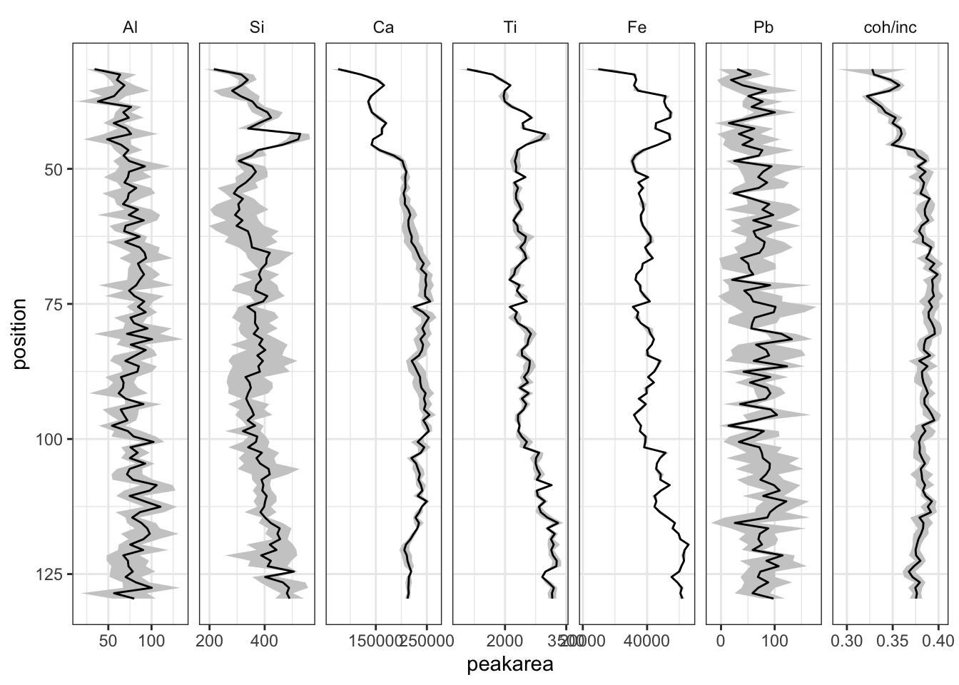

This information can be used to inform decisions about the inclusion and treatment of the remainder of the data - where there are unacceptably high uncertainties that element might be considered for exclusion from further analysis.