5.1 Ratios and Normalisation
These data are compositional, and represent the changes in the relative proportions of all components of the matrix, measured and un-measured. As such it is likely the data will need transforming for certain types of multivariate analysis. As previously mentioned, these data are dimensionless, and as such do not represent a quantity, but are directly related to the absolute amount of a particular element in the matrix. It is often the case that ratios of elements are used to represent changes in composition — this is sometimes referred to as normalisation, or normalising one element against another.
For example, particular element ratios can be used to make some environmental inference. Log-ratios are usually preferable here as they are resilient to matrix effects. In this context, the Ca/Ti log-ratio is used to infer a relative measure of productivity (that it, it can identify the hemipelagic sediments in the sequence). Note the use of abs() has the effect of ensuring that switching the denominator and numerator has no effect.
CD166_19_xrf %>%
mutate(`log(Fe/Ca)` = abs(log(Fe/Ca))) %>%
filter(qc == TRUE) %>%
ggplot(aes(x = depth, y = `log(Fe/Ca)`)) +
geom_line() +
scale_x_reverse()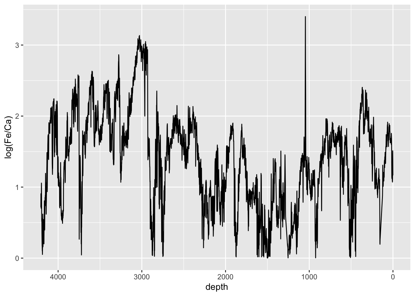 Sometimes z-scores are useful to use when units don’t have meaningful units. They scale the data in standard deviations from their mean, so give a useful quantity for the magnitude of change. For example:
CD166_19_xrf %>%
  mutate(`log(Fe/Ca)` = abs(log(Fe/Ca))) %>%
  mutate(zscore = (`log(Fe/Ca)` - mean(`log(Fe/Ca)`, na.rm = TRUE))/sd(`log(Fe/Ca)`, na.rm = TRUE)) %>%
  filter(qc == TRUE) %>%

  ggplot(aes(x = depth, y = zscore)) +
  geom_line() +
  scale_x_reverse() +
ylab("log(Fe/Ca) [z-score]") 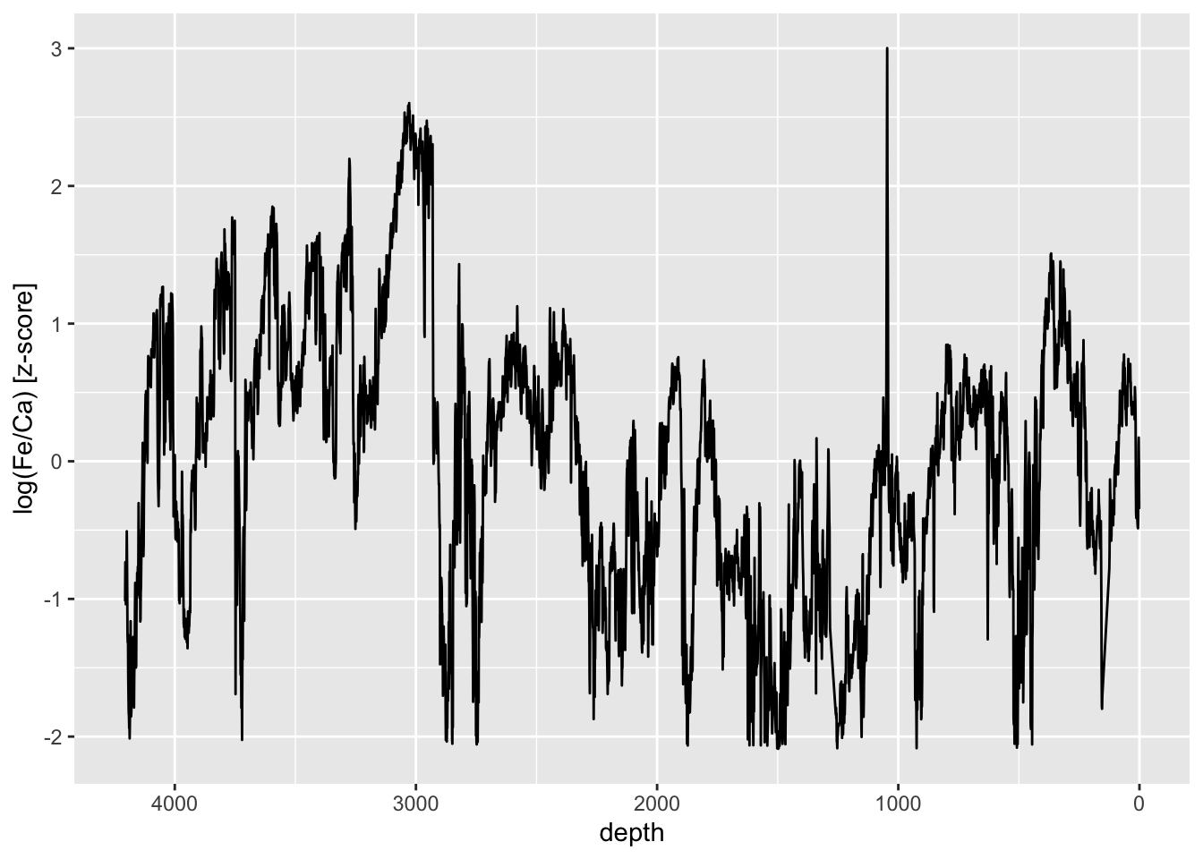
It is trivial to calculate element ratios, to the extent that these can often simply be calculated where they are required rather than saving them to memory. For example, if a plot of the Compton divided by the Rayleigh scatter was desired, there is no need to save the computed value to a new variable (e.g. coh_inc <- df$Mo.coh/df$Mo.inc) — simply define the calculation during plotting. To calculate ratios for all elements at once, use mutate(across(any_ofelementsList)), where elementsList is a list of chemical elements extracted from data(PeriodicTable).
CD166_19_xrf %>%
  mutate(across(any_of(elementsList)) /`Mo inc`)
This can be integrated into the work flow from the data tidying chapter, for example:
CD166_19_xrf %>%
  # transform
  mutate(across(any_of(elementsList)) /`Mo inc`) %>%

  # identify acceptable observations
  filter(validity == TRUE) %>%

  # identify acceptable variables
  select(any_of(myElements), depth, label) %>%

  # pivot
  tidyr::pivot_longer(!c("depth", "label"), names_to = "elements", values_to = "peakarea") %>%
  mutate(elements = factor(elements, levels = c(elementsList, "coh/inc"))) %>%

  # plot
  ggplot(aes(x = peakarea, y = depth)) +
    tidypaleo::geom_lineh(aes(color = label)) +
    scale_y_reverse() +
    scale_x_continuous(n.breaks = 2) +
    facet_geochem_gridh(vars(elements)) +
    labs(x = "peak area / Mo. inc.", y = "Depth [mm]") +
    tidypaleo::theme_paleo() +
    theme(legend.position = "none")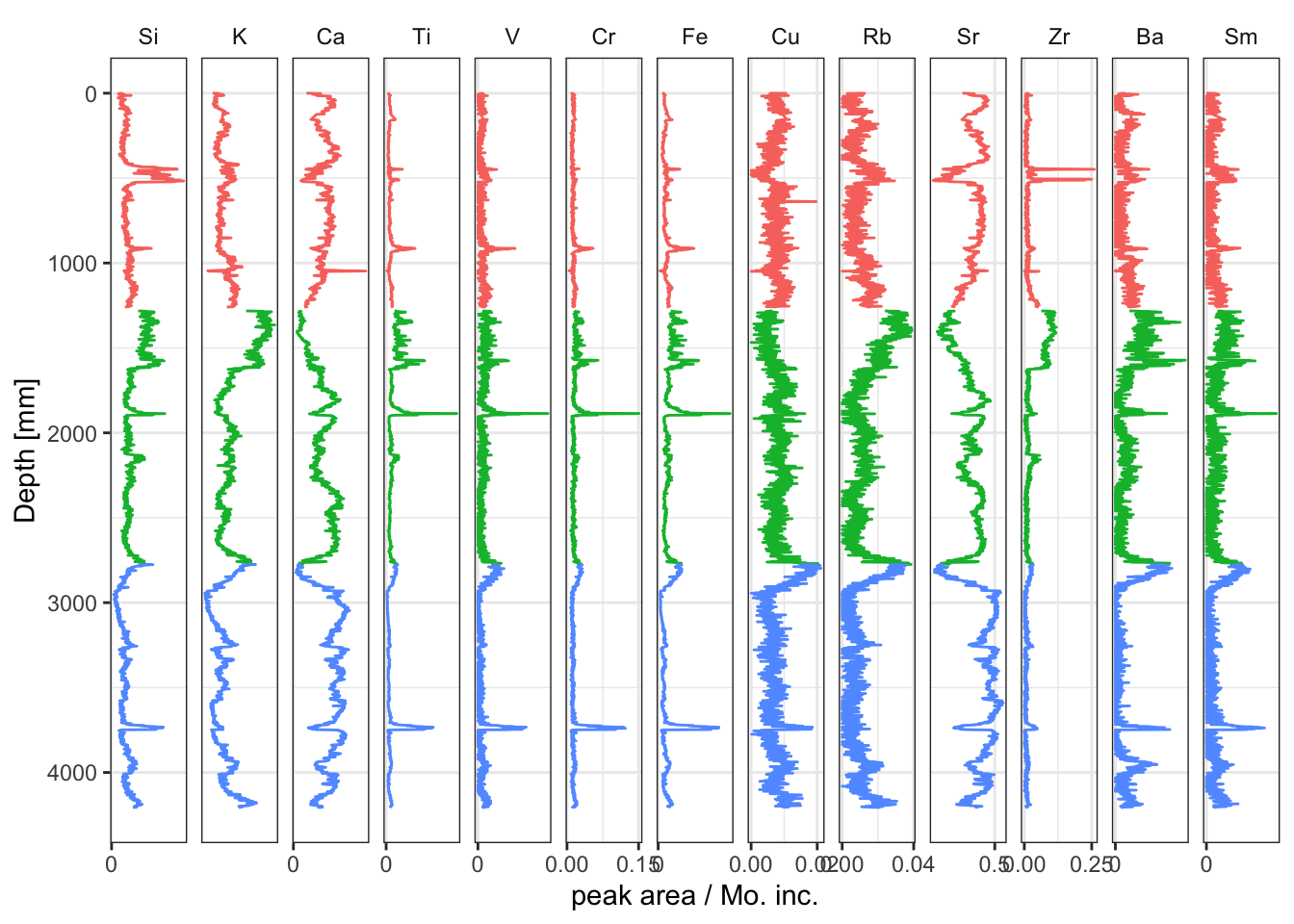
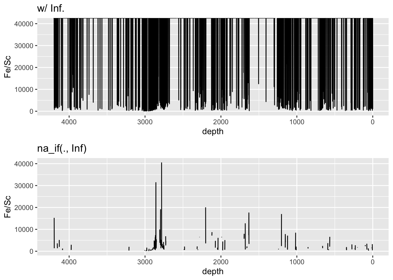
Note that where zero values are encountered in divisions, dividing by zero will lead to Inf values. This can cause issues with plotting data, and these values should be cleaned into NA before plotting. For example:
ggarrange(

  CD166_19_xrf %>%
  mutate(`Fe/Sc` = Fe/Sc) %>%
  ggplot(aes(x = depth, y = `Fe/Sc`)) +
  geom_line() +
    scale_x_reverse() +
    ggtitle("w/ Inf."),

  CD166_19_xrf %>%
  mutate(`Fe/Sc` = Fe/Sc) %>%
  mutate_if(is.numeric, list(~na_if(., Inf))) %>% # convert all Inf to NA
  ggplot(aes(x = depth, y = `Fe/Sc`)) +
  geom_line() +
    scale_x_reverse() +
    ggtitle("na_if(., Inf)")

)