7.4 Linear Methods

We’ll use our xrf and hhxrf data sets to create linear models of all the variables of interest. They must be combined using pivot_longer(). The plot indicates that some, but not all variables are suitable for calibration.

full_join(
  hhxrf %>%
    select(any_of(c(elementsList, "SampleID"))) %>%
    pivot_longer(any_of(elementsList),
                 values_to = "hhxrf",
                 names_to = "element"),
  
  xrf %>% 
    select(any_of(c(elementsList, "SampleID"))) %>%
    pivot_longer(any_of(elementsList),
                 values_to = "xrf",
                 names_to = "element"),
  
  by = c("SampleID", "element")
  ) %>%

  filter(element %in% myElements) %>%
  drop_na() %>%
  
  ggplot(aes(x = hhxrf, y = xrf)) +
  geom_point() +
  ggpmisc::stat_poly_line() +
  ggpmisc::stat_poly_eq() +
  facet_wrap(vars(element), 
             scales = "free") +
  xlab("Conventional XRF [ppm]") + 
  ylab("Itrax ED-XRF [peak area]")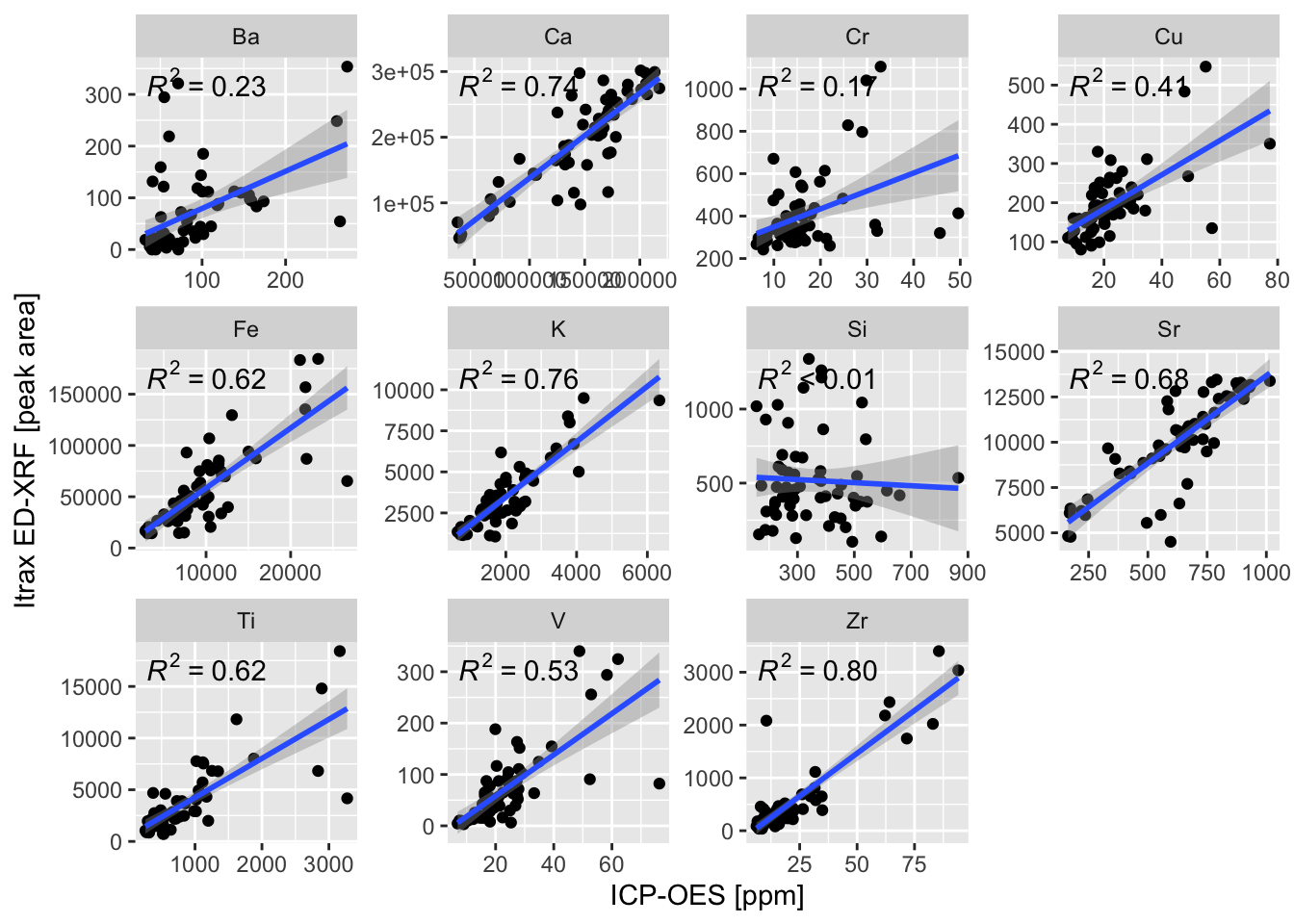

To apply these calibration models to our existing data, we first need to save the models created using lm(). We don’t force the intercept through zero (e.g. hhxrf ~ 0 + xrf) because of background (high baseline) conditions that may be present.

calibration <- full_join(
  hhxrf %>%
    select(any_of(c(elementsList, "SampleID"))) %>%
    pivot_longer(any_of(elementsList),
                 values_to = "hhxrf",
                 names_to = "element"),
  
  xrf %>% 
    select(any_of(c(elementsList, "SampleID"))) %>%
    pivot_longer(any_of(elementsList),
                 values_to = "xrf",
                 names_to = "element"),
  
  by = c("SampleID", "element")
  ) %>%
  mutate(element = as_factor(element)) %>%
  drop_na()

calibration <- calibration %>%
  group_by(element) %>%
  group_split() %>%
  lapply(function(x){lm(data = x, hhxrf~xrf)}) %>%
  `names<-`(calibration %>%
              group_by(element) %>%
              group_keys() %>%
              pull(element))

We can see the performance of our model using summary(), for example:

summary(calibration$Ca)

## Warning: In 'Ops' : non-'errors' operand automatically coerced to an 'errors'
## object with no uncertainty

## 
## Call:
## lm(formula = hhxrf ~ xrf, data = x)
## 
## Residuals:
##    Min     1Q Median     3Q    Max 
## -90606 -20066   1609  20785  76404 
## 
## Coefficients:

## Warning in printCoefmat(coefs, digits = digits, signif.stars = signif.stars, :
## NAs introduced by coercion

##                          Estimate      Std. Error        t value Pr(>|t|)    
## (Intercept) 51588.943250000(4312)  12535.14(6691)  4.11600(2242) 0.000124 ***
## xrf             0.729260000(3663) 0.0598700(3241) 12.18200(6531)  < 2e-16 ***
## ---
## Signif. codes:  0 '***' 0.001 '**' 0.01 '*' 0.05 '.' 0.1 ' ' 1
## 
## Residual standard error: 33200(200) on 58 degrees of freedom
## Multiple R-squared:  0.719,  Adjusted R-squared:  0.7141 
## F-statistic: 148.4 on 1 and 58 DF,  p-value: < 2.2e-16

Now we can use predict() to apply those models to the data.

CD166_19_xrf %>%
mutate(Ca_ppm =
         predict(calibration$Ca, 
                 newdata = 
                   CD166_19_xrf %>%
                   select(Ca) %>% 
                   rename(xrf = Ca))
       ) %>%
  ggplot(aes(x = Ca_ppm, y = depth)) +
  geom_lineh() +
  scale_y_reverse() +
  scale_x_continuous(labels = function(x){x/10000}) +
  ylab("Depth [mm]") +
  xlab("Ca [%]")

## Warning: Removed 3 rows containing missing values or values outside the scale range
## (`geom_lineh()`).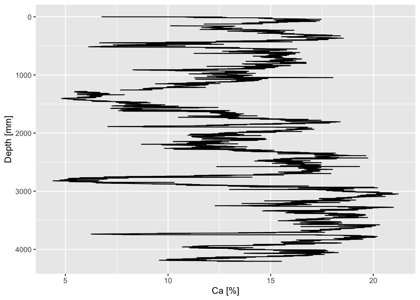

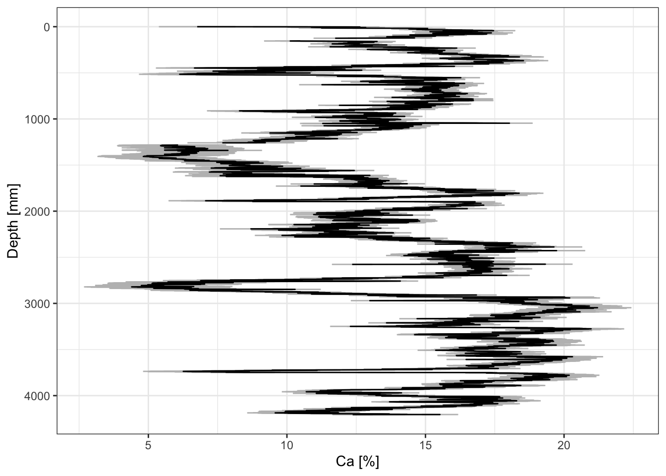
We can also extract the confidence intervals, for example:

predict(calibration$Ca, 
        newdata = 
          CD166_19_xrf %>%
          select(Ca) %>% 
          rename(xrf = Ca),
        interval = "confidence",
        level = 0.95,
        type = "response") %>%
  as_tibble() %>%
  mutate(depth = CD166_19_xrf$depth) %>%
  
  ggplot(aes(y = depth, x = fit)) +
  geom_errorbar(aes(xmin = lwr, xmax = upr), col = "grey") + 
  geom_lineh() + 
  scale_x_continuous(labels = function(x){x/10000},
                     name = "Ca [%]") +
  scale_y_reverse(name = "Depth [mm]") + 
  theme_paleo()