4.1 Plotting XRF Data

For simple biplots, ggplot2 provides the following solution. This includes different colour coding to differentiate the core sections.

ggplot(data = na.omit(CD166_19_xrf), mapping = aes(x = depth, y = `Mo coh`/`Mo inc`)) +
  geom_line(aes(color = label)) + 
  coord_flip() +
  scale_x_reverse() +
  labs(x = "Depth [mm]", color = "Core") +
  theme_classic() +
  theme(legend.position = "none")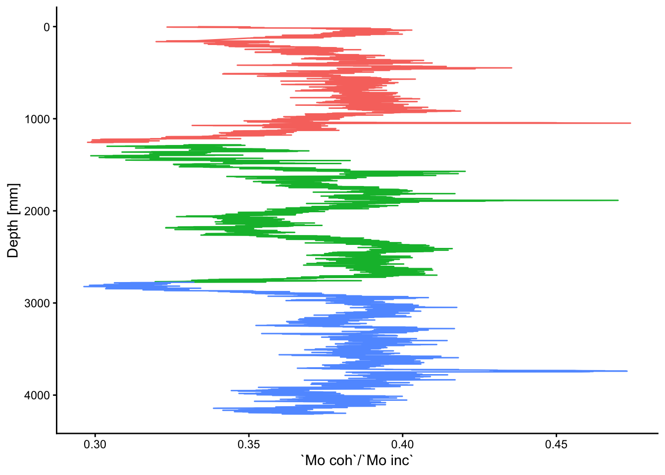

Where a traditional stratigraphic plot is desired, the tidypaleo package provides useful functionality for producing these. However, the data does need to converted to long-form from the existing table. In this way tidypaleo::facet_geochem_gridh works in a way similar to ggplot::facet_wrap but has been creates a stratigraphic plot. The elementsList is used with select(any_of()) to include only columns that are chemical elements. Depth and label are also added because they are used in the plot. Although this is useful for producing large-format summary diagrams of the data, these do not render well in smaller plot areas, so a small subset of variables has been selected manually; see the code comments below. Note that in the line mutate(), the vector passed to levels = controls the order in which the plots appear. In this example, they will appear in order of atomic weight, and the coh/inc ratio will always be last.

xrfStrat <- CD166_19_xrf %>% 
  mutate(`coh/inc` = `Mo coh`/`Mo inc`) %>%
  select(any_of(elementsList), `coh/inc`, depth, label) %>% # this is useful but produces a very large plot that doesn't render well
  select(Fe, Ti, `coh/inc`, Mn, depth, label) %>% # a smaller set of elements is defined here manually.
  tidyr::pivot_longer(!c("depth", "label"), names_to = "elements", values_to = "peakarea") %>% 
  tidyr::drop_na() %>%
  mutate(elements = factor(elements, levels = c(elementsList, "coh/inc"))) %>% # note that the levels controls the order

  ggplot(aes(x = peakarea, y = depth)) +
    tidypaleo::geom_lineh(aes(color = label)) +
    scale_y_reverse() +
    scale_x_continuous(n.breaks = 2) +
    facet_geochem_gridh(vars(elements)) +
    labs(x = "peak area", y = "Depth [mm]") +
    tidypaleo::theme_paleo() +
    theme(legend.position = "none")

print(xrfStrat)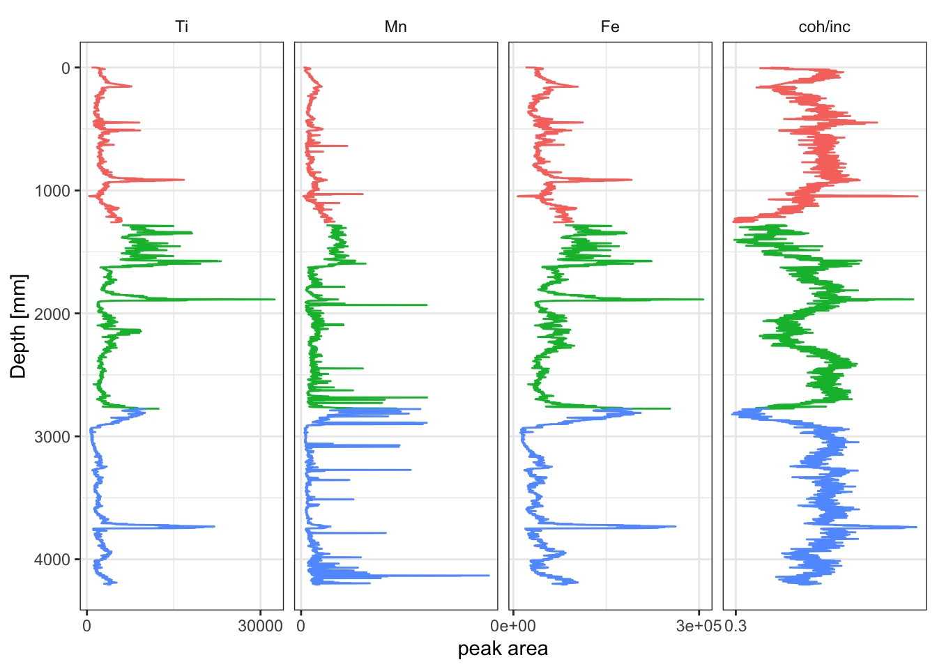

Notice that in the previous example the data must be converted to “long-form” from “short-form” for tidypaleo, using tidyr::pivot_longer. “Short-form” data has observations as rows, and variables as columns, whereas “long-form” data has a column for names, which in this case are the elements, and a column for values, in this case the peak intensities. This results in many rows, but few columns.

CD166_19_xrf %>% 
  select(any_of(elementsList), depth, label) %>%
  tidyr::pivot_longer(!c("depth", "label"), names_to = "elements", values_to = "peakarea") %>%
  glimpse()

## Rows: 151,632
## Columns: 4
## $ depth    <dbl> 0, 0, 0, 0, 0, 0, 0, 0, 0, 0, 0, 0, 0, 0, 0, 0, 0, 0, 0, 0, 0…
## $ label    <chr> "S1", "S1", "S1", "S1", "S1", "S1", "S1", "S1", "S1", "S1", "…
## $ elements <chr> "Al", "Si", "P", "S", "Cl", "Ar", "K", "Ca", "Sc", "Ti", "V",…
## $ peakarea <dbl> 41, 177, 0, 0, 726, 697, 1412, 59965, 19, 804, 26, 220, 231, …