6.2 Principal Component Analysis

Principal component analysis (PCA) is a common method for exploring multivariate data. Note the use of zeroreplace() - this is because the princomp() method defined for th acomp class uses a centred-log-ratio (clr()) transformation that is intolerant to zero-values.

CD166_19_xrf_acomp %>%
  zeroreplace() %>%
  princomp() %>%
  biplot(xlabs = rep(".",times = nrow(CD166_19_xrf_acomp)))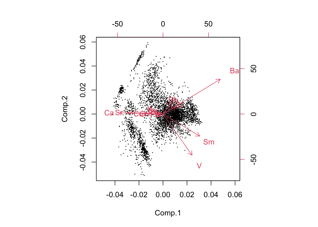

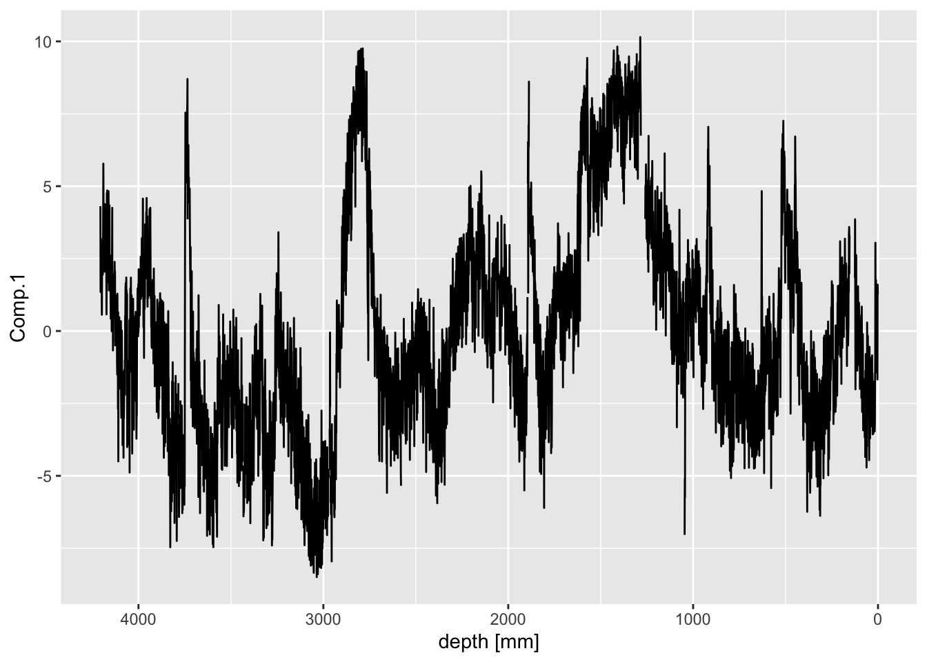
It is useful to plot components over depth. They can be extracted and plotted as follows:

bind_rows(
  tibble(depth = CD166_19_xrf %>%
           filter(qc == FALSE) %>%
           pull("depth"),
         Comp.1 = NA
        ),

  tibble(
    depth = CD166_19_xrf %>%
      filter(qc == TRUE) %>%
      pull("depth"),
    Comp.1 = CD166_19_xrf_acomp %>%
      zeroreplace() %>%
      princomp() %>%
      magrittr::extract2("scores") %>%
      as_tibble() %>%
      pull("Comp.1")
    )) %>%
  
  arrange(depth) %>%
  
  ggplot(aes(x = depth, y = Comp.1)) +
  geom_line() + 
  scale_x_reverse(name = "depth [mm]")

## Warning: Removed 4 rows containing missing values or values outside the scale range
## (`geom_line()`).