3.1 Low Count Rates

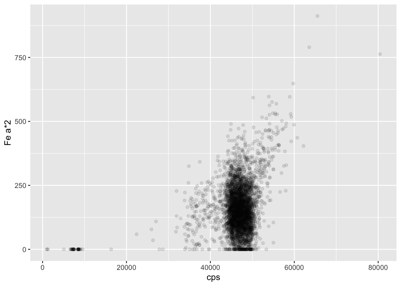
The count rate (“cps”, or counts-per-second) is the rate of energy event detection at the detector, and is a function of both the excitation beam condition (tube type, voltage and current) and the matrix. Because the tube type and voltage are often chosen based on other considerations, the operator usually only adjusts the tube current to optimise the count rate. The higher the total counts for each measurement, the better the measurement will be in terms of detection limits and uncertainties. Higher count rates allow for shorter dwell times, but this must be balanced against the need to minimise harmonics in the spectra. Harmonics can occur where the photon flux is so high that the detector cannot differentiate between two photons, and so registers the sum energy instead. For example, a particularly common phenomenon is the detection of two Fe Kα photons (energy 6.4 keV) as a single photon with the energy 12.8 keV. The graph below shows that for these cores there is the expected positive correlation between the count rate and the Fe Kα * 2 sum peak. To some extent the Q-Spec software will accommodate these harmonics, but operators commonly aim for a count rate of between 30-50 kcps.

ggplot(data = CD166_19_xrf, mapping = aes(x = cps, y = `Fe a*2`)) + 
  geom_point(alpha = 0.1) 

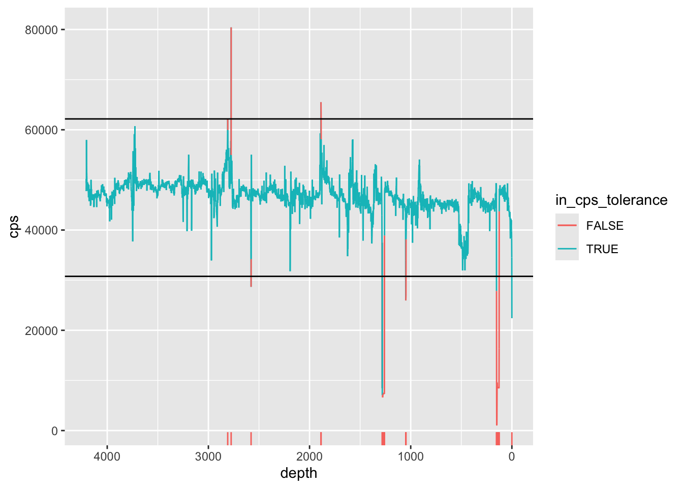
Deletion criteria can be on the basis of count rates (excluding very low and high values), selected harmonics (e.g. Fe a*2), or both. An example is shown below.

CD166_19_xrf %>%
  mutate(in_cps_tolerance = ifelse(cps <=30000 | cps >=60000 | is.na(cps) == TRUE, FALSE, TRUE)) %>%
  
  ggplot(mapping = aes(x = depth, y = cps, col = in_cps_tolerance)) + 
  geom_line(aes(group = 1)) +
  scale_x_reverse() +
  geom_hline(yintercept = c(30000, 60000)) +
  geom_rug(sides = "b", data = . %>% filter(in_cps_tolerance == FALSE)) 

It is possible, and sometimes preferable, to use some statistic to define the limits, rather than using arbitrary limits. For example, using the standard deviation (or even a confidence interval) to identify outlier data. For example:

CD166_19_xrf %>%
  mutate(in_cps_tolerance = ifelse(cps <= mean(cps)-(3*sd(cps)) | cps >=mean(cps)+(3*sd(cps)) | is.na(cps) == TRUE, FALSE, TRUE)) %>%
  
  ggplot(mapping = aes(x = depth, y = cps, col = in_cps_tolerance)) + 
  geom_line(aes(group = 1)) +
  scale_x_reverse() +
  geom_hline(yintercept = c(mean(CD166_19_xrf$cps)-(3*sd(CD166_19_xrf$cps)), mean(CD166_19_xrf$cps)+(3*sd(CD166_19_xrf$cps)))) +
  geom_rug(sides = "b", data = . %>% filter(in_cps_tolerance == FALSE))