5.2 Running Mean and Other Window Functions

Where a signal is noisy but appears to exhibit some signal it may be appropriate to use a running mean to “smooth” the signal. However, considerable caution should be exercised in the use of this tool. It is rare for an analysis to be genuinely improved by the use of running means, although it can artificially improve statistics for some tests. When visualising data using a running mean the original, unmodified data should always be shown alongside to avoid any misunderstanding. This method can be used for any suitable window function (e.g. min(), max(), range() and sd.)

CD166_19_xrf %>%
  # uses a 50 point running mean (50 mm for this data); 25 before, 25 after
  mutate(across(any_of(elementsList), 
                function(x){unlist(slider::slide(x, mean, .before = 25, .after = 25))}
                )
         ) %>%
  ggplot(mapping = aes(x = depth, y = Ca)) + 
  geom_line(data = CD166_19_xrf, col = "grey80") + 
  geom_line() + 
  scale_x_reverse() +
  theme_paleo()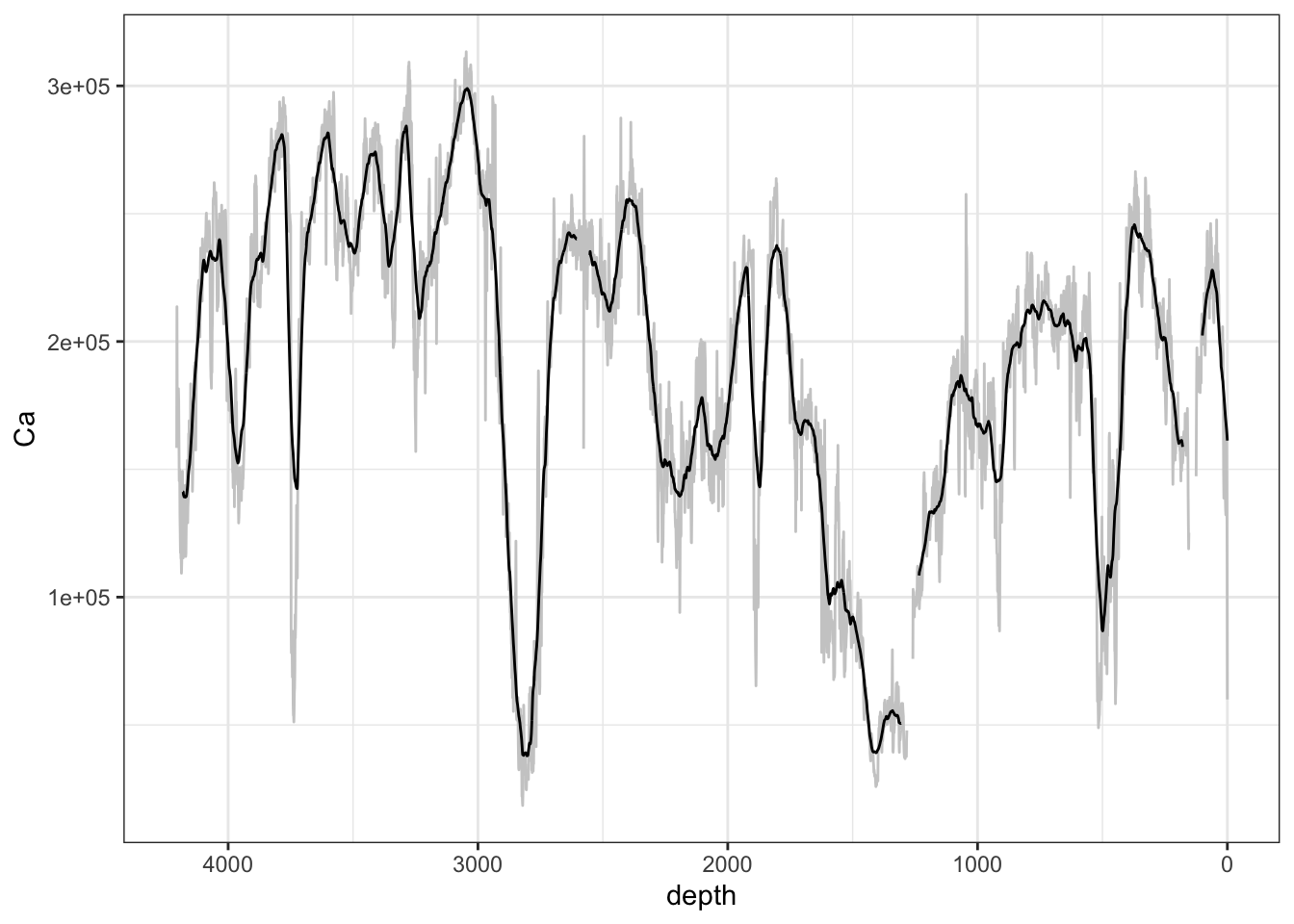

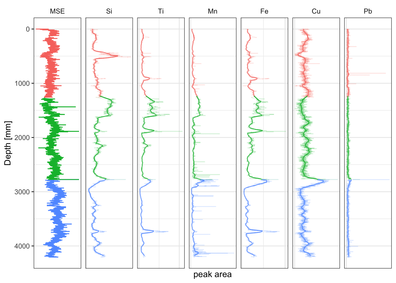
To plot the running means in a stratigraphic diagram, the smoothed data has to be labelled and combined with the original data so it can be faceted.

# make the xrf plot with running means
full_join(y = CD166_19_xrf %>%
                        as_tibble() %>%
                        # uses a 50 point running mean (50 mm for this data); 25 before, 25 after
                        mutate(across(any_of(c(elementsList)), 
                                      function(x){unlist(slider::slide(x, mean, .before = 25, .after = 25))}
                                      )
                               ) %>%
                        mutate(type = "mean"), 
                      x = CD166_19_xrf %>% 
                        as_tibble() %>% 
                        mutate(type = "raw")
                      ) %>% 
  filter(validity == TRUE) %>%
  select(Fe, Ti, Cu, Pb, Si, MSE, Mn, depth, label, type) %>%
  tidyr::pivot_longer(!c("depth", "label", "type"), names_to = "elements", values_to = "peakarea") %>% 
  tidyr::drop_na() %>%
  mutate(elements = factor(elements, levels = c("MSE", elementsList))) %>%
  mutate(label = as_factor(label),
         type = as_factor(type)
         ) %>%
  
  glimpse() %>%
  
  ggplot(aes(x = peakarea, y = depth)) +
  tidypaleo::geom_lineh(aes(group = type, colour = label, alpha = type)) +
  scale_alpha_manual(values = c(0.1, 1)) +
  scale_y_reverse() +
  scale_x_continuous(n.breaks = 2) +
  facet_geochem_gridh(vars(elements)) +
  labs(x = "peak area", y = "Depth [mm]") +
  tidypaleo::theme_paleo() +
  theme(legend.position = "none",
        axis.text.x = element_blank(),
        axis.ticks.x = element_blank())

## Rows: 57,134
## Columns: 5
## $ depth    <dbl> 0, 0, 0, 0, 0, 0, 0, 1, 1, 1, 1, 1, 1, 1, 2, 2, 2, 2, 2, 2, 2…
## $ label    <fct> S1, S1, S1, S1, S1, S1, S1, S1, S1, S1, S1, S1, S1, S1, S1, S…
## $ type     <fct> raw, raw, raw, raw, raw, raw, raw, raw, raw, raw, raw, raw, r…
## $ elements <fct> Fe, Ti, Cu, Pb, Si, MSE, Mn, Fe, Ti, Cu, Pb, Si, MSE, Mn, Fe,…
## $ peakarea <dbl> 19786.00, 804.00, 117.00, 22.00, 177.00, 1.26, 231.00, 35168.…